10.2. Further extending MUSE

10.2.1. Adding a search space filter

from muse.agents import Agent
from muse.filters import register_filter
from xarray import DataArray, Dataset


@register_filter
def no_ccgt_filter(
    agent: Agent, search_space: DataArray, technologies: Dataset, market: Dataset
) -> DataArray:
    """Excludes gasCCGT."""
    dropped_tech = search_space.where(search_space.replacement != "windturbine")
    return search_space & search_space.replacement.isin(dropped_tech.replacement)

import logging
import os

from muse import examples
from muse.mca import MCA

model_path = examples.copy_model(overwrite=True)
logging.getLogger("muse").setLevel(0)
mca = MCA.factory(os.path.join(model_path, "settings.toml"))
mca.run();

-- 2024-04-25 14:56:14 - muse.sectors.register - INFO
Sector legacy registered.

-- 2024-04-25 14:56:14 - muse.sectors.register - INFO
Sector preset registered, with alias presets.

-- 2024-04-25 14:56:14 - muse.sectors.register - INFO
Sector default registered.

import pandas as pd
import seaborn as sns

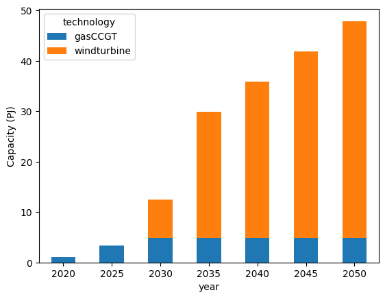
results = pd.read_csv("Results/MCACapacity.csv")
results
sns.lineplot(
    data=results[results.sector == "power"], x="year", y="capacity", hue="technology"
)

<Axes: xlabel='year', ylabel='capacity'>

10.2.2. Registering a custom decision function

Next, we would like to add an additional decision function. A decision function is a transformation applied to aggregate multiple objectives into a single objective during agent investment. For example, through the use of a weighted sum.

In this example, we would like to take the median objective. However, the functions predefined in MUSE don’t include this functionality. MUSE contains examples such as the mean, weighted sum and a single objective. Therefore we will have to register and create our own.

Now, we create our new median_objective function:

from typing import Any

from muse.decisions import register_decision
from xarray import DataArray, Dataset


@register_decision
def median_objective(objectives: Dataset, parameters: Any, **kwargs) -> DataArray:
    from xarray import concat

    allobjectives = concat(objectives.data_vars.values(), dim="concat_var")
    return allobjectives.median(set(allobjectives.dims) - {"asset", "replacement"})

After importing the decorator function, register_decision, and ensuring that we decorate our new function with @register_decision, we are able to create our new function as above.

Our new function median_objective modifies the mean function already built into MUSE, with one difference. Replacing the return value, from allobjectives.mean to allobjectives.mean.

@register_decision
def mean(objectives: Dataset, *args, **kwargs) -> DataArray:
    """Mean over objectives."""
    from xarray import concat

    allobjectives = concat(objectives.data_vars.values(), dim="concat_var")
    return allobjectives.mean(set(allobjectives.dims) - {"asset", "replacement"})

Of course, you are free to make your functions as complicated as you like, depending on your own requirements.

Next, we must edit our Agents.csv file. We will modify the default example for this tutorial. We change the first two entry rows, to be as follows:

Agent1,A1,1,R1,LCOE,NPV,EAC,1,,,TRUE,,,all,median_objective,1,-1,inf,New
Agent2,A1,2,R1,LCOE,NPV,EAC,1,,,TRUE,,,all,median_objective,1,-1,inf,Retrofit

Here, we add the NPV and EAC decision metrics, as well as replacing the singleObj DecisionMethod to median_objective.

Now we are able to run our modified model as before:

logging.getLogger("muse").setLevel(0)
mca = MCA.factory("../tutorial-code/0-new-decision-metric/settings.toml")
mca.run();

-- 2024-04-25 14:56:35 - muse.registration - WARNING
A decision with the name median_objective already exists

Again, we visualise the power sector:

import pandas as pd
import seaborn as sns

results = pd.read_csv("../tutorial-code/0-new-decision-metric/Results/MCACapacity.csv")
results = results.groupby(["year", "sector", "technology"]).sum().reset_index()
sns.lineplot(
    data=results[results.sector == "power"], x="year", y="capacity", hue="technology"
)

<Axes: xlabel='year', ylabel='capacity'>

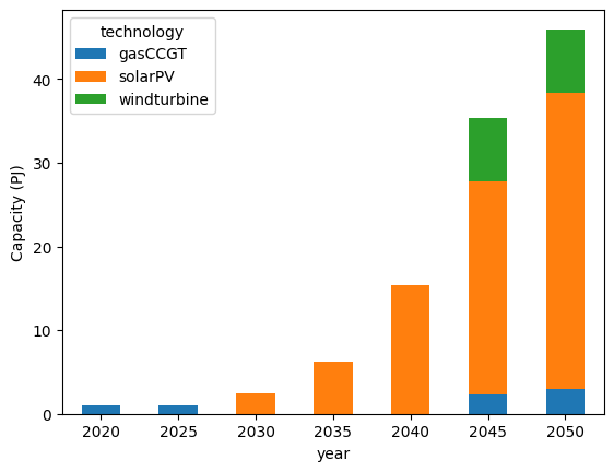
We see a different scenario emerge through these different decision metrics. This shows the importance of decision metrics when making long-term investment decisions.

10.2.3. End of tutorials

In these tutorials you have seen the ways in which you can modify MUSE. All of these methods can be combined and extended to make as simple or complex model as you wish. Feel free to experiment and come up with your own ideas for your future work!

For further information, we refer you to the API in the next section.