4. Running your first example

In this section we run an example simulation of MUSE and visualise the results. There are a number of different examples in the source code, which can be found here. Depending on how you installed MUSE, there are two scenarios for running MUSE:

• Running the model and then analysing the data separately. This is available for any of the installation methods.

• Running the model programmatically and analysing the data in the same session. This is only possible if MUSE was installed using a virtual environment, either as user or developer.

In the first case, MUSE is run with the appropriate input arguments (either using the GUI or from the command line) and then the outputs are analysed by another tool. In the tutorials we will use Jupyter (see section below for instructions on how to install it), but you can use any data analysis tool that you are comfortable with. The second case means a closer relationship between MUSE runs and the analysis tools, being able to run MUSE within a Python script with the appropriate inputs, collecting the output and analysing the results. This approach is useful to, for example, perform a parameter sweep in MUSE.

4.1. Running MUSE

Once MUSE have been installed, we can run an example. To start with, we will run one of the built-in MUSE examples. We will focus on the terminal version of MUSE as the GUI version should be largely self-explanatory. If you are using MUSE within a virtual environment, make sure you have it activated.

In all cases, if the installation instructions were followed, you should be able to run the default muse example running the following command in the terminal:

muse --model default

For the virtual environment-based ones, python -m muse --model default will also work. If running correctly, your prompt should output text similar to that which can be found here. You can check the available built-in models, as well as information on other input arguments, with:

muse -h

A common use case is to take one of the built-in models as the starting point to create your own model. This approach is used all the time in the tutorials. Just decide which model you want to use as starting point and run:

muse --model default --copy path/to/copy/the/model/to

Then, you can change the location to where you copied the example, for example Users/{my_name}/Documents/default using the cd command, or “change directory” command. Once we have navigated to the directory containing the example settings settings.toml we can run the simulation using the following command in the anaconda prompt or terminal:

muse settings.toml

4.1.1. Programmatic use of MUSE

It is also possible to run one of the built-in MUSE models directly in Python using the following code:

from muse import examples
model = examples.model("default")
model.run()

The output will be produced in the current working directory, within a Results folder. For the case of a custom settings file:

from logging import getLogger

from muse.mca import MCA
from muse.readers.toml import read_settings

settings = read_settings("/full/path/to/the/file/settings.toml")
getLogger("muse").setLevel(settings.log_level)
model = MCA.factory(settings)
model.run()

With the output being produced as indicated in the settings file.

4.2. Installing Jupyter

For the following parts of the tutorial, we will use Python to visualise the result of MUSE simulations. If you are not planning to use Jupyter for data analysis, just jump to the next section to learn how to run MUSE.

A common approach for data visualisation is to use Jupyter Notebook. Jupyter Notebook is a method of running interactive computing across dozens of programming languages. However, you are free to visualise the results using the language or program of your choice, for example Excel, R, Matlab or Python.

First, you will need to install Jupyter Notebook.

• If you already have a Python virtual environment where you installed MUSE (see section on virtual environments), you can use the same environment for Jupyter or create a separate one. If you use the same environment, you will be able to run MUSE interactively within the Jupyter Notebook.

• If you did not create a virtual environment as part of your MUSE installation (you used the Standalone or pipx-based installations), you can create and activate one now (again, see section on virtual environments)

Once your environment is activated, you can install Jupyter Notebook by following the instructions showed here. We will install the classic Jupyter Notebook, and so we will run the following code in the terminal (if you are not familiar with the terminal, check the appropriate section in the pipx-based installation):

python -m pip install jupyter

Once this has been installed you can start Jupyter Notebook by running the following command:

python -m jupyter jupyter notebook

A web browser should now open up with a URL such as the following: http://localhost:8888/tree. If it doesn’t, copy and paste the command as directed in the terminal. This will likely take the form of:

http://localhost:8888/?token=xxxxxxxxxx

With xxxxxxxxxx a very long collection of letters and numbers. Once you are on the page, you will be able to navigate to a location of your choice and create a new file, by clicking the new button in the top right, followed by clicking the Python 3 button. You should then be able to proceed and follow the tutorials in this documentation.

4.2.1. Missing packages

If when running a cell you get any errors such as:

ModuleNotFoundError: No module named 'pandas'

Then you are trying to use a package (pandas in the example) that is not available in the current environment. It is possible to install the missing packages by running the following in the jupyter notebook:

!pip install pandas

The package will be installed in whatever virtual environment Jupyter is running into.

4.3. Results

If the default MUSE example has run successfully, you should now have a folder called Results in the current working directory.

This directory should contain results for each sector (Gas,Power and Residential) as well as results for the entire simulation in the form of MCACapacity.csv and MCAPrices.csv.

• MCACapacity.csv contains information about the capacity each agent has per technology per benchmark year. Each benchmark year is the modelled year in the settings.toml file. In our example, this is 2020, 2025, …, 2050.

• MCAPrices.csv has the converged price of each commodity per benchmark year and timeslice. eg. the cost of electricity at night for electricity in 2020.

Within each of the sector result folders, there is an output for Capacity for each commodity in each year. The years into the future, which the simulation has not run to, refers to the capacity as it retires. Within the Residential folder there is also a folder for Supply within each year. This refers to how much end-use commodity was output.

The output can be fully configurable, as shown in the developer guide here.

4.4. Visualisation

import matplotlib.pyplot as plt
import pandas as pd
import seaborn as sns

Next, we load the dataset of interest to us for this example: the MCACapacity.csv file. We do this using pandas.

capacity_results = pd.read_csv("Results/MCACapacity.csv")
capacity_results.head()

	technology	dst_region	region	agent	sector	type	year	capacity
0	gasboiler	R1	R1	A1	residential	retrofit	2020	10.0
1	gasCCGT	R1	R1	A1	power	retrofit	2020	1.0
2	gassupply1	R1	R1	A1	gas	retrofit	2020	15.0
3	gasboiler	R1	R1	A1	residential	retrofit	2025	5.0
4	heatpump	R1	R1	A1	residential	retrofit	2025	19.0

Using the head command we print the first five rows of our dataset. Next, we will visualise each of the sectors, with capacity on the y-axis and year on the x-axis.

Don’t worry too much about the code if some of it is unfamiliar. We effectively split the data into each sector and then plot a line plot for each.

for sector_name, results in capacity_results.groupby("sector"):
    print("{} sector".format(sector_name))
    sns.lineplot(data=results, x="year", y="capacity", hue="technology")
    plt.ylabel("capacity (PJ)")
    plt.show()
    plt.close()

gas sector

power sector

residential sector

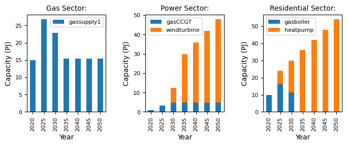
In this toy example, we can see that the end-use technology of choice in the residential sector becomes a heatpump. The heatpump displaces the gas boiler. Therefore, the supply of gas crashes due to a reduced demand. To account for the increase in demand for electricity, the agent invests heavily in wind turbines.

Note, that the units are in petajoules (PJ). MUSE requires consistent units across each of the sectors, and each of the input files (which we will see later). The model does not make any unit conversion internally.

4.5. Next steps

If you want to jump straight into customising your own example scenarios, head to the link here. If you would like a little bit of background based on how MUSE works first, head to the next section!