9.7. Production constraints by timeslice

In some sectors it may be the case that a technology can only output a certain amount at a certain time. For instance, solar photovoltaics (PV) don’t produce power in the dark, and thus their output is limited at night.

In this section, we explain how to add constraints to outputs of technologies at certain timeslices. This could either be a maximum constraint, for instance with the solar PV example previously mentioned. Or, this could be a minimum constraint, for example with a nuclear power plant, where we expect a minimum output at all times.

9.7.1. Minimum timeslice constraint

In this tutorial we will be amending the default_timeslice example.

To copy this model so you can edit the files, run:

python -m muse --model default_timeslice --copy PATH/TO/COPY/THE/MODEL/TO

You will see that, compared to the default example, this model has an additional TechnodataTimeslices.csv file in the power sector The majority of the columns in this file are self-explanatory, and correspond to the columns in other csv files - for instance, technology, region and year. The utilization_factor column specifies the maximum utilization factor for the respective technologies in the respective timeslices, and the mimimum_service_factor specifies the minimum service factor of a technology. The timeslice based columns, however, are dynamic and will match the levels as defined in the toml file.

We will modify the minimum service factor for gasCCGT in the power sector as follows.

technology	region	year	month	day	hour	utilization_factor	minimum_service_factor
gasCCGT	R1	2020	all-year	all-week	night	1	0.2
gasCCGT	R1	2020	all-year	all-week	morning	1	0.4
gasCCGT	R1	2020	all-year	all-week	afternoon	1	0.6
gasCCGT	R1	2020	all-year	all-week	early-peak	1	0.4
gasCCGT	R1	2020	all-year	all-week	late-peak	1	0.8
gasCCGT	R1	2020	all-year	all-week	evening	1	1

For example, if the capacity of gasCCGT in a given year is 1, and the minimum service factor in a timeslice is 0.5, then the minimum output in that timeslice will be capped at 0.083 (= (1 / 6) * 0.5), assuming there are 6 timeslices with equal length.

Looking at the settings.toml file, you should see that the file has already been linked to the appropriate sector:

[sectors.power]
type = 'default'
priority = 2
technodata = '{path}/power/Technodata.csv'
commodities_in = '{path}/power/CommIn.csv'
commodities_out = '{path}/power/CommOut.csv'
technodata_timeslices = '{path}/power/TechnodataTimeslices.csv'

Notice the technodata_timeslices path in the bottom row.

The default_timeslice model also includes one additional output, which gives a detailed breakdown of commodity supply in the power sector:

[[sectors.power.outputs]]
filename = "{cwd}/{default_output_dir}/{Sector}_{Quantity}.csv"
sink = "aggregate"
quantity = "supply"

This will create a new file in the results folder called Power_Supply.csv, which will be important for the analysis below.

Once you’ve had a look at these files, run MUSE with the usual command:

python -m muse settings.toml

We will then visualise the output of the technologies in each timeslice:

from pathlib import Path

import numpy as np
import pandas as pd
import seaborn as sns

def plot_supply(supply, capacity, technology, commodity, year, factor=None):
    # Plot timeslice supply
    tech_supply = (
        supply[
            (supply.technology == technology)
            & (supply.commodity == commodity)
            & (supply.year == year)
        ]
        .groupby(["timeslice", "technology"])
        .sum()
        .reset_index()
    )

    ax = sns.barplot(
        data=tech_supply,
        x="timeslice",
        y="supply",
        hue="technology",
    )
    ax.set_title(f"{commodity} supply from {technology} in {year}")

    # Add line for the expected minimum/maximum supply
    if factor is not None:
        tech_capa = capacity[
            (capacity.technology == technology) & (capacity.year == year)
        ].capacity.sum()
        min_supply = (tech_capa / 6) * factor
        ax.plot(min_supply, color="red")


path = Path("../tutorial-code/min-max-timeslice-constraints/1-min-constraint/Results/")
supply = pd.read_csv(path / "Power_Supply.csv")
capacity = pd.read_csv(path / "MCACapacity.csv")

plot_supply(
    supply,
    capacity,
    "gasCCGT",
    "electricity",
    2025,
    np.array([0.2, 0.4, 0.6, 0.4, 0.8, 1]),
)

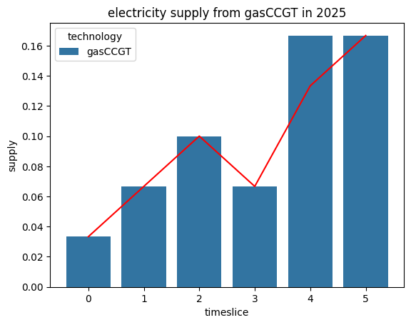
Here, we can see that the supply of electricity by gasCCGT in 2025 successfully exceeds the lower-bound cap (red line) in every timeslice.

9.7.2. Maximum timeslice constraint

Next, we will try removing the minimum constraint for the last two timeslices and instead imposing a maximum constraint using the UtilizationFactor parameter

technology	region	year	month	day	hour	utilization_factor	minimum_service_factor
gasCCGT	R1	2020	all-year	all-week	night	1	0.2
gasCCGT	R1	2020	all-year	all-week	morning	1	0.4
gasCCGT	R1	2020	all-year	all-week	afternoon	1	0.6
gasCCGT	R1	2020	all-year	all-week	early-peak	1	0.4
gasCCGT	R1	2020	all-year	all-week	late-peak	0.5	0
gasCCGT	R1	2020	all-year	all-week	evening	0.5	0

Once this has been saved, we can run the model again (python -m muse settings.toml), and visualise our results as before.

path = Path("../tutorial-code/min-max-timeslice-constraints/2-max-constraint/Results/")
supply = pd.read_csv(path / "Power_Supply.csv")
capacity = pd.read_csv(path / "MCACapacity.csv")

plot_supply(
    supply,
    capacity,
    "gasCCGT",
    "electricity",
    2025,
    np.array([1, 1, 1, 1, 0.5, 0.5]),
)

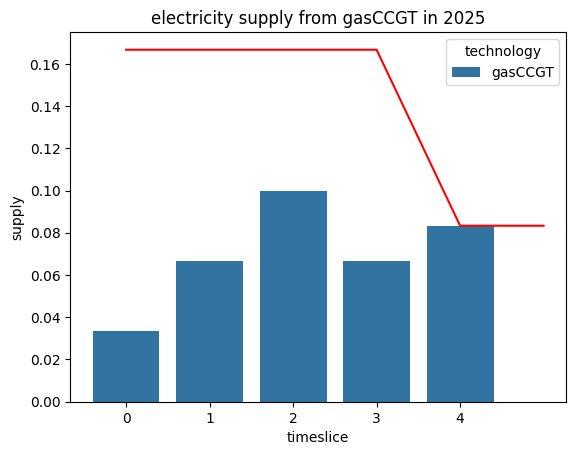
As expected, we can see an enforced reduction in supply in the final two timeslices, compared to the previous scenario.

9.7.3. Summary

In this tutorial we’ve shown had to impose minimum and maximum constraints on the activity of technologies on a timeslice-basis. Not only will this impact the supply of comodities, but it may also influence investment decisions. You are encouraged to explore the implications of this on your own.