8.6. Adding a service demand by correlation

In the previous section we added an exogenous service demand. That is, we explicitly specified what the demand would be per year.

However, we may not know what the electricity demand may be per year. Instead, we may conclude that our electricity demand is a function of the GDP and population of a particular region.

To accommodate such a scenario, MUSE enables us to choose a regression function that estimates service demands from GDP and population, which may be more certain in your case.

In this section we will show how this can be done.

8.6.1. Additional files

For this work, we will use the default example from the MUSE repository, and will not build on the previous examples. This is done to simplify the model at this point.

The full scenario files for the default example can be found here. We recommend that you download these files and save them to a location convenient to you, as we will be amending these throughout this tutorial.

Similarly to before, we must amend the preset folder for this. However, we no longer require the Residential2020Consumption.csv and Residential2050Consumption.csv files. These files set the exogenous service demand for the residential sector.

We must replace these files, with the following files:

• A macrodrivers file. This contains the drivers of the service demand that we want to model. For this example, these will include GDP based on purchasing power parity (GDP PPP) and the population that we expect from 2010 to 2110.

• A regression parameters file. This file will set the function type we would like to use to predict the service demand and the respective parameters of this regression file per region.

• A timeslice share file. This file sets how the demand is shared between timeslice.

The example files for each of those just mentioned can be found below, respectively:

• Macrodrivers.csv

• regressionparameters.csv

• TimesliceSharepreset.csv

For a full introduction to these files, see the link here.

Download these files and save them within the preset folder.

Next, we must amend our toml file to include our new way of calculating the preset service demand.

8.6.2. TOML file

Editing the TOML file to include this can be done relatively quickly if we know the variable names.

In the second bottom section of the toml file, you will see the following section:

[sectors.residential_presets]
type = 'presets'
priority = 0
consumption_path= "{path}/technodata/preset/*Consumption.csv"

This enables us to run the model in exogenous mode, but now we would like to run the model from the files previously mentioned. This can be done by linking new variables to the new files, as follows:

[sectors.residential_presets]
type = 'presets'
priority = 0

timeslice_shares_path = '{path}/technodata/preset/TimesliceSharepreset.csv'
macrodrivers_path = '{path}/technodata/preset/Macrodrivers.csv'
regression_path = '{path}/technodata/preset/regressionparameters.csv'

We effectively linked the new files to MUSE.

8.6.3. Increasing capacity constraints

Again, we must increase the capacity constraints. This is because the data in our GDP PPP and population files create a much higher demand than our previous toy example, due to the fact that it is more realistic for our particular region.

To ensure that we don’t encounter any problems, we will relax our capacity constraints considerably.

For the full files see here. Make sure to take note of the columns:

• MaxCapacityAddition

• MaxCapacityGrowth

• TotalCapacityLimit

for the Technodata.csv files for each of the sectors.

8.6.4. Running and visualising our new results

With those changes made, we are now able to run our modified model, with the python -m muse settings.toml command in anaconda prompt, as before.

As before, we will now visualise the output.

import matplotlib.pyplot as plt
import pandas as pd
import seaborn as sns

mca_capacity = pd.read_csv(
    "../tutorial-code/6-add-correlation-demand/Results/MCACapacity.csv"
)
mca_capacity.head()

	Unnamed: 0	agent	capacity	dst_region	index	installed	region	sector	technology	type	year
0	2	A1	10.0000	R1	0	2020	R1	residential	gasboiler	retrofit	2020
1	0	A1	1.0000	R1	0	2020	R1	power	gasCCGT	retrofit	2020
2	0	A1	15.0000	R1	0	2020	R1	gas	gassupply1	retrofit	2020
3	2	A1	5.0000	R1	0	2020	R1	residential	gasboiler	retrofit	2025
4	7	A1	17.4843	R1	16	2020	R1	residential	heatpump	retrofit	2025

for name, sector in mca_capacity.groupby("sector"):
    print("{} sector:".format(name))
    sns.lineplot(
        data=sector[sector.region == "R1"], x="year", y="capacity", hue="technology"
    )
    plt.show()

gas sector:

power sector:

residential sector:

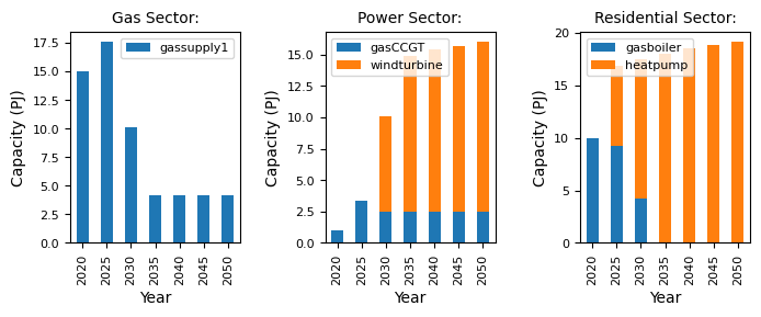
As expected, we see a scenario emerge with much higher capacity limits. The demand does not increase linearly, with variations in the total demand in the residential sector. This is due to the new function not being a linear function.

8.6.5. Next steps

In the next section we will see how we can enforce outputs of technologies by timeslice. For instance, we can prevent solar photovoltaics from producing electricity at night, or ensure that a nuclear power plant runs at a minimum capacity during the day.