8.4. Modification of time

In this section we will show you how to modify the timeslicing arrangement as well as change the time horizon and benchmark year intervals by modifying the settings.toml file.

8.4.1. Modify timeslicing

Timeslicing is the division of a single benchmark year into multiple different sections. For example, we could slice the benchmark year into different seasons, make a distinction between weekday and weekend or a distinction between morning and night. We do this as energy demand profiles can show a difference between these timeslices. eg. Electricity consumption is lower during the night than during the day.

To achieve this, we have to modify the settings.toml file, as well as the files within the preset folder: Residential2020Consumption.csv and Residential2050Consumption.csv. This is so that we can edit the demand for the residential sector for the new timeslices.

First we edit the settings.toml file to add two additional timeslices: early-morning and late-afternoon. We also rename afternoon to mid-afternoon. These settings can be found at the bottom of the settings.toml file.

An example of the changes is shown below:

[timeslices]
all-year.all-week.night = 1095
all-year.all-week.morning = 1095
all-year.all-week.mid-afternoon = 1095
all-year.all-week.early-peak = 1095
all-year.all-week.late-peak = 1095
all-year.all-week.evening = 1095
all-year.all-week.early-morning = 1095
all-year.all-week.late-afternoon = 1095
level_names = ["month", "day", "hour"]

The number of timeslices within this should add up to 8760; the number of hours in a benchmark year. Whilst this is required, MUSE does not check and enforce this.

Next, we modify both Residential Consumption files. Again, we put the text in bold for the modified entries. We must add the demand for the two additional timelsices, which we call timeslice 7 and 8. We make the demand for heat to be 2 for both of the new timeslices.

Below is the modified Residential2020Consumption.csv file:

	RegionName	ProcessName	Timeslice	electricity	gas	heat	CO2f	wind
0	R1	gasboiler	1	0	0	1	0	0
1	R1	gasboiler	2	0	0	1.5	0	0
2	R1	gasboiler	3	0	0	1	0	0
3	R1	gasboiler	4	0	0	1.5	0	0
4	R1	gasboiler	5	0	0	3	0	0
5	R1	gasboiler	6	0	0	2	0	0
6	R1	gasboiler	7	0	0	2	0	0
7	R1	gasboiler	8	0	0	2	0	0
0	R2	gasboiler	1	0	0	1	0	0
1	R2	gasboiler	2	0	0	1.5	0	0
2	R2	gasboiler	3	0	0	1	0	0
3	R2	gasboiler	4	0	0	1.5	0	0
4	R2	gasboiler	5	0	0	3	0	0
5	R2	gasboiler	6	0	0	2	0	0
6	R2	gasboiler	7	0	0	2	0	0
7	R2	gasboiler	8	0	0	2	0	0

The ProcessName must be reported, but it is not binding on the results. It is just the way that the model reads the input data.

We do the same for the Residential2050Consumption.csv, however this time we make the demand for heat in 2050 to both be 5 for the new timeslices. See here for the full file.

Once the relevant files have been edited, we are able to run the simulation model using python -m muse settings.toml.

Then, once run, we import the necessary packages:

import matplotlib.pyplot as plt
import pandas as pd
import seaborn as sns

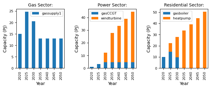
and visualise the relevant data:

mca_capacity = pd.read_csv(
    "../tutorial-code/4-modify-timing-data/1-modify-timeslices/Results/MCACapacity.csv"
)

for name, sector in mca_capacity.groupby("sector"):
    print("{} sector:".format(name))
    g = sns.FacetGrid(data=sector, col="region")
    g.map(sns.lineplot, "year", "capacity", "technology")
    g.add_legend()
    plt.show()
    plt.close()

gas sector:

power sector:

residential sector:

Compared to the scenario where we added a region, there is a smaller increase in solarPV in region R2 in the power sector. However, the rest remains largely unchanged.

This example shows the trade-off between time granularity and speed of computation. This is due to the fact that as we add more timesteps, the model takes longer to run, but slightly different scenarios emerge. It is up to you to decide what level of granularity is required for your use case.

8.4.2. Modify time horizon and time periods

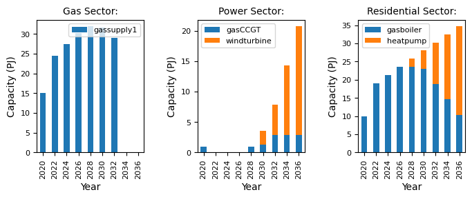
For the previous examples, we have run the scenario from 2020 to 2050, in 5 year time steps per benchmark year. This has been set at the top of the settings.toml file. However, we may want to run a more detailed scenario, with 2 year time steps, and up until the year 2040.

Making this change is quite simple as we only have two lines to change. We will modify line 2 and 3 of the settings.toml file, as follows:

# Global settings - most REQUIRED
time_framework = [2020, 2022, 2024, 2026, 2028, 2030, 2032, 2034, 2036, 2038, 2040]
foresight = 2   # Has to be a multiple of the minimum separation between the benchmark years

The time_framework details each benchmark year in which we run the simulation. The foresight variable details how much foresight an agent has when making investments.

As we have modified the timeslicing arrangements there will be a change in the underlying demand for heating. This may require more electricity to service this demand. Therefore, we relax the constraints for growth in the power sector for all technologies and constraints in the technodata/power/technodata.csv, as shown below:

ProcessName	RegionName	…	MaxCapacityAddition	MaxCapacityGrowth	TotalCapacityLimit	…	Agent1
Unit		…	PJ	%	PJ	…	New
gasCCGT	R1	…	40	0.2	120	…	0
windturbine	R1	…	40	0.2	120	…	0
solarPV	R1	…	40	0.2	120	…	0
gasCCGT	R2	…	40	0.2	120	…	0
windturbine	R2	…	40	0.2	120	…	0
solarPV	R2	…	40	0.2	120	…	0
…	…	…	…	…	…	…	…

We also modify the constraints defined in the technodata.csv file for the residential sector, as shown below.

ProcessName	RegionName	Time	…	MaxCapacityAddition	MaxCapacityGrowth	TotalCapacityLimit	…	Agent1
Unit		Year	…	PJ	%	PJ	…	New
gasboiler	R1	2020	…	60	0.5	120	…	0
heatpump	R1	2020	…	60	0.5	120	…	0
gasboiler	R2	2020	…	60	0.5	120	…	0
heatpump	R2	2020	…	60	0.5	120	…	0

It must be noted, that this is a toy example. For modelling a real life scenario, data should be sought to ensure that these constraints remain realistic.

For the full power sector technodata.csv file click here, and for the full residential sector technodata.csv file click here.

mca_capacity = pd.read_csv(
    "../tutorial-code/4-modify-timing-data/2-modify-time-framework/Results/MCACapacity.csv"
)

for name, sector in mca_capacity.groupby("sector"):
    print("{} sector:".format(name))
    g = sns.FacetGrid(data=sector, col="region")
    g.map(sns.lineplot, "year", "capacity", "technology")
    g.add_legend()
    plt.show()
    plt.close()

gas sector:

power sector:

residential sector:

Through the addition of more benchmark years, we are able to see a different scenario develop.

8.4.3. Next steps

In the next section we detail how to add an exogenous service demand, such as demand for heating or cooking.