9.4. Adding an agent

This tutorial will show how we can add additional agents to the model, and modify the objectives of these agents.

Again, we will build off the default model that comes with MUSE. To copy the files for this model, run:

python -m muse --model default --copy PATH/TO/COPY/THE/MODEL/TO

We will begin by adding a second agent to this model. Compared to the current agent, which bases investment decisions on minimising LCOE, the second agent will aim to minimise fuel consumption costs.

9.4.1. Creating an agent

To create the new agent, we must first modify the Agents.csv file in the directory:

{PATH_TO_MODEL}/Agents.csv

To start with, we will copy the data for agent A1 to create a new agent A2, and we will change the objective of this agent to fuel_consumption_cost. We keep obj_sort1 as True, which indicates that the objective should be minimised, rather than maximised. Also notice that we amend the quantity column, to specify that each agent makes up 50% of the population.

Again, we only show some of the columns due to space constraints, however see here for the full file.

agent_share	name	region	objective1	obj_data1	…	decision_method	quantity	type
Agent1	A1	R1	LCOE	1	…	singleObj	0.5	New
Agent2	A2	R1	fuel_consumption_cost	1	…	singleObj	0.5	New

We then edit all of the Technodata files to split the existing capacity between the two agents by the proportions we like. As we now have two agents which take up 50% of the population each, we will split the existing capacity by 50% for each of the agents.

The new technodata file for the power sector should look like the following:

technology	region	year	cap_par	cap_exp	…	Agent1	Agent2
gasCCGT	R1	2020	23.78234399	1	…	0.5	0.5
windturbine	R1	2020	36.30771182	1	…	0.5	0.5

Remember you will have to make the same changes for the residential and gas sectors!

We will now save this file and run the new simulation model using the following command:

python -m muse settings.toml

Again, we use seaborn and pandas to analyse the data in the Results folder.

import matplotlib.pyplot as plt
import pandas as pd
import seaborn as sns

mca_capacity = pd.read_csv(
    "../tutorial-code/add-agent/1-single-objective/Results/MCACapacity.csv"
)
mca_capacity.head()

	agent	capacity	dst_region	installed	region	sector	technology	type	year
0	A1	5.0	r1	2020	r1	residential	gasboiler	newcapa	2020
1	A2	5.0	r1	2020	r1	residential	gasboiler	newcapa	2020
2	A1	0.5	r1	2020	r1	power	gasCCGT	newcapa	2020
3	A2	0.5	r1	2020	r1	power	gasCCGT	newcapa	2020
4	A1	7.5	r1	2020	r1	gas	gassupply1	newcapa	2020

This time we can see that there is data for the new agent, A2. Next, we will visualise the investments made by each of the agents using seaborn’s facetgrid command. For simplicity, we will only visualise the residential sector.

mca_capacity = pd.read_csv(
    "../tutorial-code/add-agent/1-single-objective/Results/MCACapacity.csv"
)
sector_data = mca_capacity[mca_capacity["sector"] == "residential"]
sector_capacity = (
    sector_data.groupby(["year", "agent", "technology"]).sum().reset_index()
)
g = sns.FacetGrid(data=sector_capacity, col="agent")
g.map_dataframe(
    lambda data, **kwargs: data.pivot(
        index="year", columns="technology", values="capacity"
    ).plot(kind="bar", stacked=True, ax=plt.gca())
)
g.add_legend()
g.set_ylabels("Capacity (PJ)")
g.figure.suptitle("Residential Sector:")
g.figure.subplots_adjust(top=0.8)

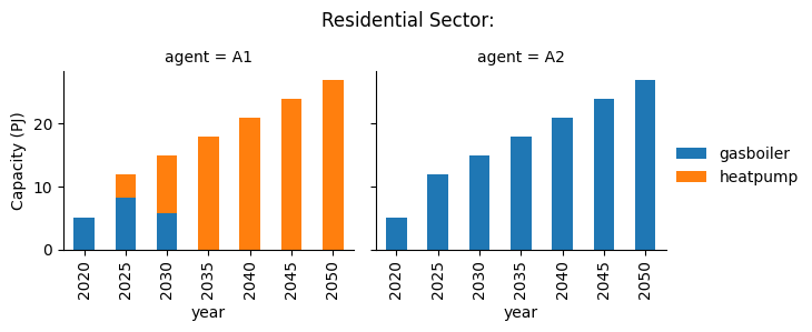
We can see different results between the two agents. Whilst agent A1 invests heavily in heat pumps, agent A2 invests entirely in gas boilers, due to the lower fuel costs of this technology.

9.4.2. Combining multiple objectives

We can also use multiple objectives for a single agent, combining objectives by taking a weighted sum. We will try this for agent A2, using both fuel_consumption_cost and LCOE with relative weights of 0.5 each.

To do this, we need to add the new objective in the objective2 column, use obj_sort2 to indicate that this objective should be minimised, modify decision_method to indicate that a weighted sum should be taken between the two objectives, and specify the weights of the two objectives in obj_data1 and obj_data2:

agent_share	name	region	objective1	objective2	obj_data1	obj_data2	…	obj_sort2	…	decision_method	quantity	type
Agent1	A1	R1	LCOE		1		…		…	singleObj	0.5	New
Agent2	A2	R1	fuel_consumption_cost	LCOE	0.5	0.5	…	True	…	weighted_sum	0.5	New

We will then re-run the simulation, and visualise the results as before:

mca_capacity = pd.read_csv(
    "../tutorial-code/add-agent/2-multiple-objective/Results/MCACapacity.csv"
)
sector_data = mca_capacity[mca_capacity["sector"] == "residential"]
sector_capacity = (
    sector_data.groupby(["year", "agent", "technology"]).sum().reset_index()
)
g = sns.FacetGrid(data=sector_capacity, col="agent")
g.map_dataframe(
    lambda data, **kwargs: data.pivot(
        index="year", columns="technology", values="capacity"
    ).plot(kind="bar", stacked=True, ax=plt.gca())
)
g.add_legend()
g.set_ylabels("Capacity (PJ)")
g.figure.suptitle("Residential Sector:")
g.figure.subplots_adjust(top=0.8)

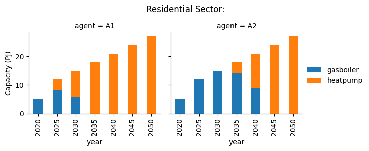
In this scenario we can see that agent A2 has an intermediate behaviour compared to the two agents in the first simulation, investing in both gas boilers and heat pumps.

9.4.3. Summary

From this small scenario, the difference between investment strategies between agents is evident. This is one of the key benefits of agent-based models when compared to optimisation-based models.

Have a play around with the files to see if you can come up with different scenarios!