9.1. Adding a new technology
In this tutorial we will begin by giving an overview of the input files that MUSE requires to run. We will then show how to modify these files to add a new technology to the model.
9.1.1. Input Files
MUSE is made up of a number of different input files. These can be broadly split into two types:
Simulation settings specify how a simulation should be run. For example, which sectors to run, for how many years, the benchmark years and what to output. In this context, benchmark years are the years in which the model is solved. In the examples following, we solve for every 5 years (ie. 2020, 2025, 2030 etc.) Simulation data, on the other hand, parametrises the technologies involved in the simulation, or the number and kinds of agents. To create a customised case study it is necessary to edit both of these file types. Simulation settings are specified in a TOML file. TOML is a simple, extensible and intuitive file format well suited for specifying small sets of complex data. Simulation data is specified in CSV files. This is a common format used for larger datasets, and is made up of columns and rows, with a comma used to differentiate between entries.
MUSE requires at least the following files to successfully run:
a single simulation settings TOML file for the simulation as a whole
a file indicating initial market price projections
a file describing the commodities in the simulation
for generalized sectors:
a file descring the agents
a file descring the technologies
a file descring the input commodities for each technology
a file descring the output commodities for each technology
a file descring the existing capacity of a given sector
for each preset sector:
a csv file describing consumption for the duration of the simulation
For a full description of these files see the input files section.
9.1.2. Copying the default model
MUSE contains an inbuilt default model with three energy sectors (gas, power and electricity), and a preset sector containing residential demands for heating. In this tutorial we will supplement this model by adding an additional power technology: solar photovoltaics (solarPV).
The first step is to create a copy of the default model files:
python -m muse --model default --copy PATH/TO/COPY/THE/MODEL/TO
You will see that the resulting folder contains a settings.toml file, a folder for each sector, and a few top-level csv files for cross-sector simulation data. In the rest of this tutorial we will edit these files to add a new technology to the simulation. You can modify the files in your favourite spreadsheet editor or text editor such as VSCODE, Excel, Numbers, Notepad or TextEdit.
9.1.3. Adding a solar commodity to the model
The new technology will consume solar energy and output electricity. As we do not already have a commodity in the model describing solar energy, we need to add this. To do so, open up the GlobalCommodities.csv file and add the following row (in bold):
commodity |
commodity_type |
unit |
|---|---|---|
electricity |
Energy |
PJ |
gas |
Energy |
PJ |
heat |
Energy |
PJ |
wind |
Energy |
PJ |
CO2f |
Environmental |
kt |
solar |
Energy |
PJ |
We specify the units as PJ and the commodity type as “Energy” (as opposed to “Environmental” which is used for non-energy polutants such as CO2)
9.1.4. Adding a solarPV technology
Next, we will open up the Technodata.csv file for the power sector. This contains parametrisation data for the technologies in the sector, such as costs, growth constraints and lifetime. MUSE allows us to vary these parameters by year, but we can also just specify parameters for the first year and MUSE will carry these forward to future years, as we’ve done below:
technology |
region |
year |
cap_par |
cap_exp |
… |
Agent1 |
|---|---|---|---|---|---|---|
gasCCGT |
R1 |
2020 |
23.78234399 |
1 |
… |
1 |
windturbine |
R1 |
2020 |
36.30771182 |
1 |
… |
1 |
solarPV |
R1 |
2020 |
30 |
1 |
… |
1 |
To create a new solarPV technology, add the row highlighted in bold above. (We are only displaying the some of the due to space constraints. The remaining parameters will be copied from the windturbine technology. You can see the full file here, and details about each parameter here.)
Next, we will use the CommIn.csv and CommOut.csv files to specify the input and output commodites of the technology. In the case of the CommIn.csv file, we add a new row for solarPV and specify a fixed input quantity of 1 for solar. Neither gasCCGT nor windturbine consume solar, so we set solar input to zero for these technologies:
technology |
region |
year |
Level |
gas |
wind |
solar |
|---|---|---|---|---|---|---|
gasCCGT |
R1 |
2020 |
fixed |
1.67 |
0 |
0 |
windturbine |
R1 |
2020 |
fixed |
0 |
1 |
0 |
solarPV |
R1 |
2020 |
fixed |
0 |
0 |
1 |
For the CommOut.csv file, we want the output of electricity to be 1 (it doesn’t emit any CO2 so we set this column to zero):
technology |
region |
year |
electricity |
CO2f |
|---|---|---|---|---|
gasCCGT |
R1 |
2020 |
1 |
91.67 |
windturbine |
R1 |
2020 |
1 |
0 |
solarPV |
R1 |
2020 |
1 |
0 |
Finally, we will modify the ExistingCapacity.csv file. This file details the existing capacity of each technology, and a decommissioning profile across every year of the time framework. For this example, we will set the existing capacity to be 0.
ProcessName |
RegionName |
2020 |
2025 |
2030 |
2035 |
2040 |
2045 |
2050 |
|---|---|---|---|---|---|---|---|---|
gasCCGT |
R1 |
1 |
1 |
0 |
0 |
0 |
0 |
0 |
windturbine |
R1 |
0 |
0 |
0 |
0 |
0 |
0 |
0 |
solarPV |
R1 |
0 |
0 |
0 |
0 |
0 |
0 |
0 |
9.1.5. Settings file
Finally, we must make a small change to the settings.toml file. As solar is a renewable resource that isn’t produced by any process defined in the model, we must add it to excluded_commodities in settings.toml, like so:
excluded_commodities = ["wind", "solar"]
This will ensure MUSE excludes solar from its internal supply-fulfillment checks.
9.1.6. Running our customised simulation
Now we are able to run our simulation with the new solar power technology. To do this, we run the following command in the command line:
python -m muse settings.toml
If the simulation has run successfully, you should now have a folder in the same location as your settings.toml file called Results. The next step is to visualise the results using the data analysis library pandas and the plotting library matplotlib.
[1]:
import matplotlib.pyplot as plt
import pandas as pd
First, we will import the MCACapacity.csv file using pandas, and print the first 5 lines with the head() command. (Make sure to change the file path as appropriate.)
[2]:
mca_capacity = pd.read_csv(
    "../tutorial-code/add-new-technology/1-introduction/Results/MCACapacity.csv"
)
mca_capacity.head()
[2]:
| agent | capacity | dst_region | installed | region | sector | technology | type | year | |
|---|---|---|---|---|---|---|---|---|---|
| 0 | A1 | 10.0000 | r1 | 2020 | r1 | residential | gasboiler | newcapa | 2020 |
| 1 | A1 | 1.0000 | r1 | 2020 | r1 | power | gasCCGT | newcapa | 2020 |
| 2 | A1 | 15.0000 | r1 | 2020 | r1 | gas | gassupply1 | newcapa | 2020 |
| 3 | A1 | 5.0000 | r1 | 2020 | r1 | residential | gasboiler | newcapa | 2025 |
| 4 | A1 | 11.4063 | r1 | 2025 | r1 | residential | gasboiler | newcapa | 2025 |
We will now visualise the results:
[3]:
fig, axes = plt.subplots(1, 3)
all_years = mca_capacity["year"].unique()
for ax, (sector_name, sector_data) in zip(axes, mca_capacity.groupby("sector")):
    sector_capacity = sector_data.groupby(["year", "technology"]).sum().reset_index()
    sector_capacity.pivot(
        index="year", columns="technology", values="capacity"
    ).reindex(all_years).plot(kind="bar", stacked=True, ax=ax)
    ax.set_ylabel("Capacity (PJ)")
    ax.set_xlabel("Year")
    ax.set_title(f"{sector_name.capitalize()} Sector:", fontsize=10)
    ax.legend(title=None, prop={"size": 8})
    ax.tick_params(axis="both", labelsize=8)

fig.set_size_inches(8, 2.5)
fig.subplots_adjust(wspace=0.5)
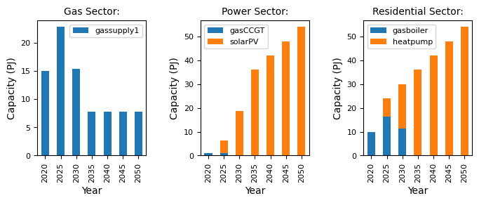
We can now see that there is solarPV capacity in the power sector. That’s great and means it worked!
We can see that solarPV has a higher uptake than gasCCGT, and has entirely replaced windturbine in the sector, which is likely due to the lower cap_par (capital cost) which makes it more favourable for investment. We can investigate this by changing the cap_par value for solarPV, which we will do in the next section.
9.1.7. Changing the capital costs of solarPV
Now, we will observe what happens if we increase the capital price of solar to be more expensive than wind in the year 2020, but then reduce the price of solar in 2040. By doing this, we should observe an initial investment in wind in the first few benchmark years of the simulation, followed by a transition to solar as we approach the year 2040.
To achieve this, we have to modify the Technodata.csv file in the power sector.
ProcessName |
RegionName |
Time |
cap_par |
cap_exp |
… |
Agent1 |
|---|---|---|---|---|---|---|
gasCCGT |
R1 |
2020 |
23.78234399 |
1 |
… |
1 |
gasCCGT |
R1 |
2040 |
23.78234399 |
1 |
… |
1 |
windturbine |
R1 |
2020 |
36.30771182 |
1 |
… |
1 |
windturbine |
R1 |
2040 |
36.30771182 |
1 |
… |
1 |
solarPV |
R1 |
2020 |
100 |
1 |
… |
1 |
solarPV |
R1 |
2040 |
30 |
1 |
… |
1 |
Here, we increase cap_par for solarPV to 100 in the year 2020, and create a new row for 2040 with a reduced cap_par of 30.
MUSE uses interpolation for the years which are unknown. So in this example, for the benchmark years between 2020 and 2040 (2025, 2030, 2035), MUSE uses interpolated cap_par values. The interpolation mode can be set in the settings.toml file, and defaults to linear interpolation. This example uses the default setting for interpolation.
Note that we must also provide entries for 2040 for the other technologies, gasCCGT and windturbine. For this example, we will keep these the same as before, copying and pasting the rows.
We can now rerun the simulation, using the same command as previously, import the new MCACapacity.csv file again, and visualise the results:
[4]:
mca_capacity = pd.read_csv(
    "../tutorial-code/add-new-technology/2-scenario/Results/MCACapacity.csv"
)

fig, axes = plt.subplots(1, 3)
all_years = mca_capacity["year"].unique()
for ax, (sector_name, sector_data) in zip(axes, mca_capacity.groupby("sector")):
    sector_capacity = sector_data.groupby(["year", "technology"]).sum().reset_index()
    sector_capacity.pivot(
        index="year", columns="technology", values="capacity"
    ).reindex(all_years).plot(kind="bar", stacked=True, ax=ax)
    ax.set_ylabel("Capacity (PJ)")
    ax.set_xlabel("Year")
    ax.set_title(f"{sector_name.capitalize()} Sector:", fontsize=10)
    ax.legend(title=None, prop={"size": 8})
    ax.tick_params(axis="both", labelsize=8)

fig.set_size_inches(8, 2.5)
fig.subplots_adjust(wspace=0.5)
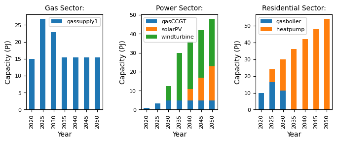
From the results, we can see that some of the early solarPV investment has been replaced by windturbine. However, in later years, as the capital cost of solarPV decreases, the share of solarPV begins to increase.
For the full example with the completed input files see here.
9.1.8. Summary
In this tutorial we have shown how to add a new technology to the model, and how to modify the parameters of this technology. Have a go at modifying some of the other parameters to see how this affects investment decisions.