8.5. Adding a region

This tutorial will show you how to add additional regions to the model.

Again, we will build off the default model that comes with MUSE. To copy the files for this model, run:

python -m muse --model default --copy PATH/TO/COPY/THE/MODEL/TO

We will add a region called R2 (however, this could equally be called USA or India). This requires us to undertake a similar process as before of modifying the input simulation data.

8.5.1. Input files

We begin by modifying the settings.toml file. We just have to add our new region to the regions variable, in the 4th line of the file, like so:

regions = ["R1", "R2"]

The process to change the input files, however, takes a bit more time. To achieve this, there must be data for each of the sectors for the new region. This, therefore, requires the modification of every input file.

Due to space constraints, we will not show you how to edit all of the files. However, you can access the modified files here.

Effectively, for this example, we will copy and paste the rows in each of the input files from region R1, and change the name of the region for the new rows to R2.

We have placed two examples as to how to edit the residential sector below. Again, the edited data are highlighted in bold, with the original data in normal text.

The following file is the modified /residential/CommIn.csv file:

ProcessName	RegionName	Time	Level	electricity	gas	heat	CO2f	wind
Unit		Year		PJ/PJ	PJ/PJ	PJ/PJ	kt/PJ	PJ/PJ
gasboiler	R1	2020	fixed	0	1.16	0	0	0
heatpump	R1	2020	fixed	0.4	0	0	0	0
gasboiler	R2	2020	fixed	0	1.16	0	0	0
heatpump	R2	2020	fixed	0.4	0	0	0	0
…	…	…	…	…	…	…	…	…

Whereas the following file is the modified /residential/ExistingCapacity.csv file:

ProcessName	RegionName	Unit	2020	2025	2030	2035	2040	2045	2050
gasboiler	R1	PJ/y	10	5	0	0	0	0	0
heatpump	R1	PJ/y	0	0	0	0	0	0	0
gasboiler	R2	PJ/y	10	5	0	0	0	0	0
heatpump	R2	PJ/y	0	0	0	0	0	0	0

We will follow a similar process in the /residential/Technodata.csv file, copying the lines from R1 to create R2. In this tutorial we will test the scenario where heatpump has a strict upper limit on total capacity in R2, using the TotalCapacityLimit parameter, which is highlighted below in bold. The rest of the elements are the same for R1 as they are for R2.

ProcessName	RegionName	Time	…	TotalCapacityLimit	…	Agent1
Unit		Year	…	PJ	…	New
gasboiler	R1	2020	…	100	…	1
heatpump	R1	2020	…	100	…	1
gasboiler	R2	2020	…	100	…	1
heatpump	R2	2020	…	20	…	1

Now, go ahead and amend all of the other input files for each of the sectors (including the preset sector, which defines the residential commodity demand in each region) by copying and pasting the rows from R1 and replacing the RegionName to R2 for the new rows. You must also modify the Projections.csv file in the input folder in a similar way.

All of the edited input files can be seen here.

8.5.2. Results

Again, we will run the results using the python -m pip muse settings.toml in the command line, and visualize the data as follows:

import matplotlib.pyplot as plt
import pandas as pd
import seaborn as sns

mca_capacity = pd.read_csv(
    "../tutorial-code/add-region/1-new-region/Results/MCACapacity.csv"
)
all_years = mca_capacity["year"].unique()

for sector_name, sector_data in mca_capacity.groupby("sector"):
    sector_capacity = (
        sector_data.groupby(["year", "region", "technology"]).sum().reset_index()
    )
    g = sns.FacetGrid(data=sector_capacity, col="region")
    g.map_dataframe(
        lambda data, **kwargs: data.pivot(
            index="year", columns="technology", values="capacity"
        )
        .reindex(all_years)
        .plot(kind="bar", stacked=True, ax=plt.gca())
    )
    g.add_legend()
    g.set_ylabels("Capacity (PJ)")
    g.figure.suptitle(f"{sector_name.capitalize()} Sector:")
    g.figure.subplots_adjust(top=0.8)

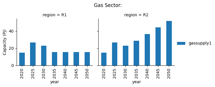
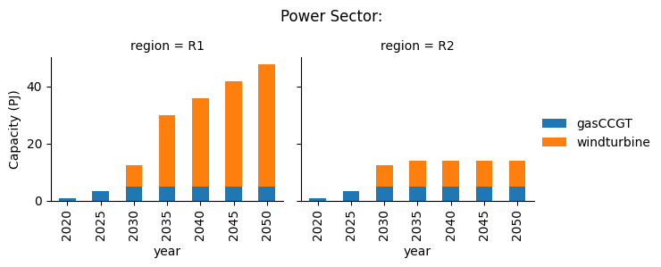
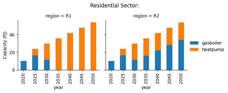
We can see that R2 quickly reaches its capacity limit for heatpump, and additional investment in gasboiler needed to meet the residential heating demand.

8.5.3. Summary

In this tutorial we have shown how to add a new region to the model, and shown how the TotalCapacityLimit parameter can be used to put an upper limit on capacity in a region.

Have a play around with the various costs data in the technodata files for each of the sectors and technologies to see if different scenarios emerge. Although be careful. In some cases, the constraints on certain technologies will make it impossible for the demand to be met and it will give you an error such as the following:

message: 'The algorithm terminated successfully and determined that the problem is infeasible.'

To avoid this error message you may have to relax the constraints in the technodata files (MaxCapacityGrowth, MaxCapacityAddition and TotalCapacityLimit)