8.2. Adding a service demand

In this section, we detail how to add a service demand to MUSE. In the residential sector, a service demand could be cooking. Houses require energy to cook food and a technology to service this demand, such as an electric stove. This process consists of setting a demand, either through inputs derived from the user or correlations of GDP and population which reflect the socioeconomic development of a region or country. In addition, a technology must be added to service this new demand.

This tutorial will build off the default model that comes with MUSE. To copy the files for this model, run:

python -m muse --model default --copy PATH/TO/COPY/THE/MODEL/TO

8.2.1. Addition of cooking demand

In this example, we will add a cooking preset demand. To achieve this, we will first edit the Residential2020Consumption.csv and Residential2050Consumption.csv files, found within the residential_presets directory.

The Residential2020Consumption.csv file allows us to specify the demand in 2020 for each region and technology per timeslice. The Residential2050Consumption.csv file does the same, but for the year 2050. The datapoints between these years are interpolated.

Firstly, we must add the new service demand, cook, to these two files, with values specifying the demand. For simplicity, we will copy over the values from the heat column:

RegionName	Timeslice	electricity	gas	heat	CO2f	wind	cook
R1	1	0	0	1.0	0	0	1.0
R1	2	0	0	1.5	0	0	1.5
R1	3	0	0	1.0	0	0	1.0
R1	4	0	0	1.5	0	0	1.5
R1	5	0	0	3.0	0	0	3.0
R1	6	0	0	2.0	0	0	2.0

The process is very similar for the Residential2050Consumption.csv file: again we copy the values over from the heat column. For the complete file see the link here.

Next, we must edit the GlobalCommodities.csv file (in the input folder). This is where we define the new commodity cook. It tells MUSE the commodity type, name, emissions factor of CO2 and heat rate, amongst other things:

Commodity	CommodityType	CommodityName	CommodityEmissionFactor_CO2	HeatRate	Unit
Electricity	Energy	electricity	0	1	PJ
Gas	Energy	gas	56.1	1	PJ
Heat	Energy	heat	0	1	PJ
Wind	Energy	wind	0	1	PJ
CO2fuelcomsbustion	Environmental	CO2f	0	1	kt
Cook	Energy	cook	0	1	PJ

Finally, the Projections.csv file must be changed. This is a large file which details the expected cost of the commodities across the timeframe of the simulation. Due to its size, we will only show two rows of the new column cook:

RegionName	Attribute	Time	…	cook
Unit		Year	…	MUS$2010/PJ
R1	CommodityPrice	2010	…	100
…	…	…	…	…
R1	CommodityPrice	2100	…	100

We set every price of cook to be 100MUS$2010/PJ

8.2.2. Addition of cooking technology

Next, we must add a technology to service this new demand. This is similar to how we added the solarPV technology in a previous tutorial. However, we must be careful to specify the end-use of the technology as cook.

For this example, we will add two competing technologies to service the cooking demand (electric_stove and gas_stove) to the residential/Technodata.csv file.

Again, in the interests of space, we have omitted the existing gasboiler and heatpump technologies. For the new electric_stove technology, we will copy and paste the data from the heatpump row. For gas_stove, we copy and paste the data for gasboiler. Importantly, however, we must specify the end-use for these new technologies to be cook and not heat:

ProcessName	RegionName	Time	cap_par	…	Agent1
Unit		Year	MUS$2010/PJ_a	…	New
…	…	…	…	…	…
electric_stove	R1	2020	8.8667	…	1
gas_stove	R1	2020	3.8	…	1

As can be seen, we have added two technologies with different cap_par costs. We specified their respective fuels, and the enduse for both is cook. For the full file please see here.

We must also add the data for these new technologies to the following files:

• CommIn.csv

• CommOut.csv

• ExistingCapacity.csv

This is largely a similar process to the previous tutorial. We must add the input to each of the technologies (gas and electricity for gas_stove and electric_stove respectively), outputs of cook for both and the existing capacity for each technology in each region.

To prevent repetition of the previous tutorial, we will leave the full files here.

Again, we run the simulation with our modified input files using the following command, in the relevant directory:

python -m muse settings.toml

Once this has run we are ready to visualise our results.

import matplotlib.pyplot as plt
import pandas as pd

mca_capacity = pd.read_csv(
    "../tutorial-code/add-service-demand/1-exogenous-demand/Results/MCACapacity.csv"
)
mca_capacity.head()

	agent	capacity	dst_region	installed	region	sector	technology	type	year
0	A1	10.0000	R1	2020	R1	residential	gas_stove	newcapa	2020
1	A1	10.0000	R1	2020	R1	residential	gasboiler	newcapa	2020
2	A1	1.0000	R1	2020	R1	power	gasCCGT	newcapa	2020
3	A1	15.0000	R1	2020	R1	gas	gassupply1	newcapa	2020
4	A1	7.5938	R1	2025	R1	residential	electric_stove	newcapa	2025

fig, axes = plt.subplots(1, 3)
all_years = mca_capacity["year"].unique()
for ax, (sector_name, sector_data) in zip(axes, mca_capacity.groupby("sector")):
    sector_capacity = sector_data.groupby(["year", "technology"]).sum().reset_index()
    sector_capacity.pivot(
        index="year", columns="technology", values="capacity"
    ).reindex(all_years).plot(kind="bar", stacked=True, ax=ax)
    ax.set_ylabel("Capacity (PJ)")
    ax.set_xlabel("Year")
    ax.set_title(f"{sector_name.capitalize()} Sector:", fontsize=10)
    ax.legend(title=None, prop={"size": 8})
    ax.tick_params(axis="both", labelsize=8)

fig.set_size_inches(8, 2.5)
fig.subplots_adjust(wspace=0.5)

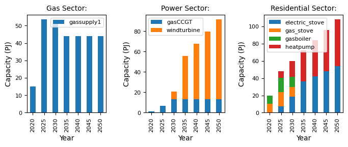
We can see that electric_stove is heavily used in the residential sector, and gas_stove is barely used at all. Therefore, compared to the default model, there is a larger increase in capacity in the power sector to accommodate this increase in demand for electricity, which is largely driven by windturbine.

8.2.3. Summary

In this tutorial we have shown how to add a service demand to MUSE, and how to add technologies to meet this demand. Try changing the demand profile for cook to see how this influences investment decisions.