8.1. Adding a new technology
In this tutorial we will begin by giving an overview of the input files that MUSE requires to run. We will then show how to modify these files to add a new technology to the model.
8.1.1. Input Files
MUSE is made up of a number of different input files. These can be broadly split into two types:
Simulation settings specify how a simulation should be run. For example, which sectors to run, for how many years, the benchmark years and what to output. In this context, benchmark years are the years in which the model is solved. In the examples following, we solve for every 5 years, ie. 2020, 2025, 2030…
Simulation data, on the other hand, parametrises the technologies involved in the simulation, or the number and kinds of agents.
To create a customised case study it is necessary to edit both of these file types.
Simulation settings are specified in a TOML file. TOML is a simple, extensible and intuitive file format well suited for specifying small sets of complex data.
Simulation data is specified in CSV files. This is a common format used for larger datasets, and is made up of columns and rows, with a comma used to differentiate between entries.
MUSE requires at least the following files to successfully run:
a single simulation settings TOML file for the simulation as a whole
a file indicating initial market price projections
a file describing the commodities in the simulation
for generalized sectors:
a file descring the agents
a file descring the technologies
a file descring the input commodities for each technology
a file descring the output commodities for each technology
a file descring the existing capacity of a given sector
for each preset sector:
a csv file describing consumption for the duration of the simulation
For a full description of these files see the input files section. To see how to customise an example, continue on this page.
8.1.2. Addition of solar PV
In this section, we will add solar photovoltaics to the default model. To achieve this, we must modify some of the input files shown in the above section. To create a copy of the default model files, run:
python -m muse --model default --copy PATH/TO/COPY/THE/MODEL/TO
You can modify the files in your favourite spreadsheet editor or text editor such as VSCODE, Excel, Numbers, Notepad or TextEdit.
8.1.3. Technodata Input
Within the default folder you’ll find a settings.toml file, input folder and technodata folder. To add a technology within the power sector, we must open the technodata folder followed by the power folder.
At this point, we must note that we require consistency in input and output units. For example, if capacity is in PJ, the same basis would be needed for the output files CommIn.csv and CommOut.csv. In addition, across sectors a commodity needs to maintain the same unit. In these examples, we use the unit petajoule (PJ).
We will first edit the CommIn.csv file, which specifies the commodities consumed by solar photovoltaics.
The table below shows the original CommIn.csv version in normal text, and the added column and row in bold.
ProcessName |
RegionName |
Time |
Level |
electricity |
gas |
heat |
CO2f |
wind |
solar |
|---|---|---|---|---|---|---|---|---|---|
Unit |
Year |
PJ/PJ |
PJ/PJ |
PJ/PJ |
kt/PJ |
PJ/PJ |
PJ/PJ |
||
gasCCGT |
R1 |
2020 |
fixed |
0 |
1.67 |
0 |
0 |
0 |
0 |
windturbine |
R1 |
2020 |
fixed |
0 |
0 |
0 |
0 |
1 |
0 |
solarPV |
R1 |
2020 |
fixed |
0 |
0 |
0 |
0 |
0 |
1 |
We must first add a new row at the bottom of the file, to indicate the new solar photovoltaic technology:
we call this technology
solarPVplace it in region
R1the data in this row is associated to the year 2020
the input type is fixed
solarPV consumes solar
As the solar commodity has not been previously defined, we must define it by adding a column, which we will call solar. We fill out the entries in the solar column, ie. that neither gasCCGT nor windturbine consume solar.
We repeat this process for the file: CommOut.csv. This file specifies the output of the technology. In our case, solar photovoltaics only output electricity. This is unlike gasCCGT which also outputs CO2f (carbon dioxide).
ProcessName |
RegionName |
Time |
electricity |
gas |
heat |
CO2f |
wind |
solar |
|---|---|---|---|---|---|---|---|---|
Unit |
Year |
PJ/PJ |
PJ/PJ |
PJ/PJ |
kt/PJ |
PJ/PJ |
PJ/PJ |
|
gasCCGT |
R1 |
2020 |
1 |
0 |
0 |
91.67 |
0 |
0 |
windturbine |
R1 |
2020 |
1 |
0 |
0 |
0 |
0 |
0 |
solarPV |
R1 |
2020 |
1 |
0 |
0 |
0 |
0 |
0 |
Similar to the the CommIn.csv, we create a new row, and add in the solar commodity. We must ensure that we call our new commodity and technologies the same as the previous file for MUSE to successfully run. ie solar and solarPV. Please note that we use flat forward extension of the values when only one value is defined. For example, in the CommOut.csv we only provide data for the year 2020. Therefore for the benchmark years, 2025, 2030, 2035… we assume the data remains
unchanged from 2020.
The next file to modify is the ExistingCapacity.csv file. This file details the existing capacity of each technology, and a decommissioning profile across the time framework. For this example, we will set the existing capacity to be 0. Please note that the model interpolates linearly between years.
ProcessName |
RegionName |
Unit |
2020 |
2025 |
2030 |
2035 |
2040 |
2045 |
2050 |
|---|---|---|---|---|---|---|---|---|---|
gasCCGT |
R1 |
PJ/y |
1 |
1 |
0 |
0 |
0 |
0 |
0 |
windturbine |
R1 |
PJ/y |
0 |
0 |
0 |
0 |
0 |
0 |
0 |
solarPV |
R1 |
PJ/y |
0 |
0 |
0 |
0 |
0 |
0 |
0 |
Finally, the Technodata.csv file contains parametrisation data for the technology, such as the cost, growth constraints, lifetime of the power plant and fuel used. We will only display the some of the parameters, as the table is too large to display in full. The remaining parameters will be copied from the windturbine technology. You can see the full file
here, and details about each parameter here.
ProcessName |
RegionName |
Time |
cap_par |
cap_exp |
… |
Agent1 |
|---|---|---|---|---|---|---|
Unit |
Year |
MUS$2010/PJ_a |
… |
New |
||
gasCCGT |
R1 |
2020 |
23.78234399 |
1 |
… |
1 |
windturbine |
R1 |
2020 |
36.30771182 |
1 |
… |
1 |
solarPV |
R1 |
2020 |
30 |
1 |
… |
1 |
Again, flat forward extension is used. Therefore, as we only provide data for the benchmark year 2020, 2025 and the following benchmark years will keep the same characteristics.
8.1.4. Global inputs
Next, navigate to the input folder. We must now edit each of the files found here to add the new solar commodity. Due to space constraints we will not display all of the entries contained in every input. You can be view the edited files in full here.
Commodities are defined in the GlobalCommodities.csv file. Here we give the commodities a commodity type, CO2 emissions factor and heat rate. For this file, we will add the solar commodity, with zero CO2 emissions factor and a heat rate of 1.
Commodity |
CommodityType |
CommodityName |
CommodityEmissionFactor_CO2 |
HeatRate |
Unit |
|---|---|---|---|---|---|
Electricity |
Energy |
electricity |
0 |
1 |
PJ |
Gas |
Energy |
gas |
56.1 |
1 |
PJ |
Heat |
Energy |
heat |
0 |
1 |
PJ |
Wind |
Energy |
wind |
0 |
1 |
PJ |
CO2fuelcomsbustion |
Environmental |
CO2f |
0 |
1 |
kt |
Solar |
Energy |
solar |
0 |
1 |
PJ |
The Projections.csv file details the initial market prices for the commodities. The market clearing algorithm will update these throughout the simulation, however an initial estimate is required to start the simulation. As solar energy is free, we will indicate this by adding a final column. Please note that the unit row is not read by MUSE, but used as a reference for the user. The units should be consistent across all input files for MUSE; MUSE does not carry out any unit conversion.
RegionName |
Attribute |
Time |
electricity |
gas |
heat |
CO2f |
wind |
solar |
|---|---|---|---|---|---|---|---|---|
Unit |
Year |
MUS$2010/PJ |
MUS$2010/PJ |
MUS$2010/PJ |
MUS$2010/kt |
MUS$2010/PJ |
MUS$2010/PJ |
|
R1 |
CommodityPrice |
2010 |
14.81481472 |
6.6759 |
100 |
0 |
0 |
0 |
R1 |
CommodityPrice |
2015 |
17.89814806 |
6.914325 |
100 |
0.052913851 |
0 |
0 |
… |
… |
… |
… |
… |
… |
… |
… |
… |
R1 |
CommodityPrice |
2100 |
21.39814806 |
7.373485819 |
100 |
1.871299697 |
0 |
0 |
It is also possible to model import and export of commodities, using the BaseYearImport.csv and BaseYearExport.csv files, along with the base_year_import and base_year_import settings in the settings file. However we will not do this here.
8.1.5. Settings
Finally, we must make a small change to the settings.toml file. As solar is a renewable resource that isn’t produced by any process defined in the model, we must add it to excluded_commodities in settings.toml, like so:
excluded_commodities = ["wind", "solar"]
This will ensure MUSE excludes solar from its internal supply-fulfillment checks.
8.1.6. Running our customised simulation
Now we are able to run our simulation with the new solar power technology. To do this, we run the following command in the command line:
python -m muse settings.toml
If the simulation has run successfully, you should now have a folder in the same location as your settings.toml file called Results. The next step is to visualise the results using the data analysis library pandas and the plotting library matplotlib.
[1]:
import matplotlib.pyplot as plt
import pandas as pd
First, we will import the MCACapacity.csv file using pandas, and print the first 5 lines with the head() command. (Make sure to change the file path as appropriate.)
[2]:
mca_capacity = pd.read_csv(
    "../tutorial-code/add-new-technology/1-introduction/Results/MCACapacity.csv"
)
mca_capacity.head()
[2]:
| agent | capacity | dst_region | installed | region | sector | technology | type | year | |
|---|---|---|---|---|---|---|---|---|---|
| 0 | A1 | 10.0000 | R1 | 2020 | R1 | residential | gasboiler | newcapa | 2020 |
| 1 | A1 | 1.0000 | R1 | 2020 | R1 | power | gasCCGT | newcapa | 2020 |
| 2 | A1 | 15.0000 | R1 | 2020 | R1 | gas | gassupply1 | newcapa | 2020 |
| 3 | A1 | 5.0000 | R1 | 2020 | R1 | residential | gasboiler | newcapa | 2025 |
| 4 | A1 | 11.4063 | R1 | 2025 | R1 | residential | gasboiler | newcapa | 2025 |
We will now visualise the results:
[3]:
fig, axes = plt.subplots(1, 3)
all_years = mca_capacity["year"].unique()
for ax, (sector_name, sector_data) in zip(axes, mca_capacity.groupby("sector")):
    sector_capacity = sector_data.groupby(["year", "technology"]).sum().reset_index()
    sector_capacity.pivot(
        index="year", columns="technology", values="capacity"
    ).reindex(all_years).plot(kind="bar", stacked=True, ax=ax)
    ax.set_ylabel("Capacity (PJ)")
    ax.set_xlabel("Year")
    ax.set_title(f"{sector_name.capitalize()} Sector:", fontsize=10)
    ax.legend(title=None, prop={"size": 8})
    ax.tick_params(axis="both", labelsize=8)

fig.set_size_inches(8, 2.5)
fig.subplots_adjust(wspace=0.5)
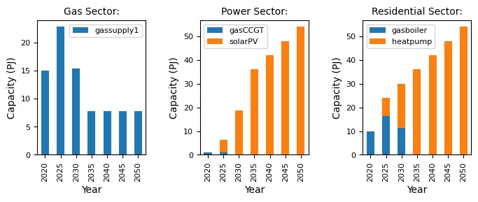
We can now see that there is solarPV capacity in the power sector. That’s great and means it worked!
We can see that solarPV has a higher uptake than gasCCGT, and has entirely replaced windturbine in of the sector, which is likely due to the lower cap_par (capital cost) which makes it more favourable for investment. We can investigate this by changing the cap_par value for solarPV, which we will do in the next section.
8.1.7. Change Capital costs of Solar
Now, we will observe what happens if we increase the capital price of solar to be more expensive than wind in the year 2020, but then reduce the price of solar in 2040. By doing this, we should observe an initial investment in wind in the first few benchmark years of the simulation, followed by a transition to solar as we approach the year 2040.
To achieve this, we have to modify the Technodata.csv, CommIn.csv and CommOut.csv files in the power sector.
First, we will amend the Technodata.csv file as follows:
ProcessName |
RegionName |
Time |
cap_par |
cap_exp |
… |
Agent1 |
|---|---|---|---|---|---|---|
Unit |
Year |
MUS$2010/PJ_a |
… |
New |
||
gasCCGT |
R1 |
2020 |
23.78234399 |
1 |
… |
1 |
gasCCGT |
R1 |
2040 |
23.78234399 |
1 |
… |
1 |
windturbine |
R1 |
2020 |
36.30771182 |
1 |
… |
1 |
windturbine |
R1 |
2040 |
36.30771182 |
1 |
… |
1 |
solarPV |
R1 |
2020 |
40 |
1 |
… |
1 |
solarPV |
R1 |
2040 |
30 |
1 |
… |
1 |
Here, we increase cap_par for solarPV to 40 in the year 2020, and create a new row for 2040 with a reduced cap_par of 30.
MUSE uses interpolation for the years which are unknown. So in this example, for the benchmark years between 2020 and 2040 (2025, 2030, 2035), MUSE uses interpolated cap_par values. The interpolation mode can be set in the settings.toml file, and defaults to linear interpolation. This example uses the default setting for interpolation.
Note that we must also provide entries for 2040 for the other technologies, gasCCGT and windturbine. For this example, we will keep these the same as before, copying and pasting the rows.
Next we will modify the CommIn.csv file.
For this step, we have to provide the input commodities for each technology, in each of the years defined in the Technodata.csv file. So, for this example, we are required to provide entries for the years 2020 and 2040 for each of the technologies. For now, we won’t change the 2040 values compared to the 2020. Therefore, we just need to copy and paste each of the entries for each of the technologies, as shown below:
ProcessName |
RegionName |
Time |
Level |
electricity |
gas |
heat |
CO2f |
wind |
solar |
|---|---|---|---|---|---|---|---|---|---|
Unit |
Year |
PJ/PJ |
PJ/PJ |
PJ/PJ |
kt/PJ |
PJ/PJ |
PJ/PJ |
||
gasCCGT |
R1 |
2020 |
fixed |
0 |
1.67 |
0 |
0 |
0 |
0 |
gasCCGT |
R1 |
2040 |
fixed |
0 |
1.67 |
0 |
0 |
0 |
0 |
windturbine |
R1 |
2020 |
fixed |
0 |
0 |
0 |
0 |
1 |
0 |
windturbine |
R1 |
2040 |
fixed |
0 |
0 |
0 |
0 |
1 |
0 |
solarPV |
R1 |
2020 |
fixed |
0 |
0 |
0 |
0 |
0 |
1 |
solarPV |
R1 |
2040 |
fixed |
0 |
0 |
0 |
0 |
0 |
1 |
We must do the same for the CommOut.csv file. For the sake of brevity we won’t show you this, but the link to the file can be found here.
We will now rerun the simulation, using the same command as previously, import the new MCACapacity.csv file again, and visualise the results:
[4]:
mca_capacity = pd.read_csv(
    "../tutorial-code/add-new-technology/2-scenario/Results/MCACapacity.csv"
)

fig, axes = plt.subplots(1, 3)
all_years = mca_capacity["year"].unique()
for ax, (sector_name, sector_data) in zip(axes, mca_capacity.groupby("sector")):
    sector_capacity = sector_data.groupby(["year", "technology"]).sum().reset_index()
    sector_capacity.pivot(
        index="year", columns="technology", values="capacity"
    ).reindex(all_years).plot(kind="bar", stacked=True, ax=ax)
    ax.set_ylabel("Capacity (PJ)")
    ax.set_xlabel("Year")
    ax.set_title(f"{sector_name.capitalize()} Sector:", fontsize=10)
    ax.legend(title=None, prop={"size": 8})
    ax.tick_params(axis="both", labelsize=8)

fig.set_size_inches(8, 2.5)
fig.subplots_adjust(wspace=0.5)
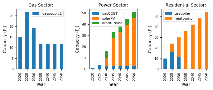
From the results, we can see that windturbine now outcompetes solarPV in the year 2025. However, between the years 2025 and 2050, as the capital cost of solarPV decreases, the share of solarPV begins to increase.
For the full example with the completed input files see here.
8.1.8. Summary
In this tutorial we have shown how to add a new technology to the model, and how to modify the parameters of this technology. Have a go at modifying some of the other parameters to see how this affects investment decisions.