9.8. Using a carbon budget

This tutorial will show how to use a carbon budget to limit carbon emissions.

Again, we will build off the default model that comes with MUSE. To copy the files for this model, run:

python -m muse --model default --copy PATH/TO/COPY/THE/MODEL/TO

9.8.1. Adding a carbon budget

Using a carbon budget allows the carbon price to be escalated (if necessary), to encourage investment in low-carbon technologies and bring emissions down in line with the budget. To achieve this, MUSE must solve the system with a number of different carbon prices in every year to uncover the relationship between carbon price and emissions. This will most likely be a monotonically decreasing function (i.e. lower emissions as carbon price increases), but may be highly non-linear and discontinuous. By building a picture of this landscape by repeatedly sampling different carbon prices, MUSE can select the carbon price that gives emissions as close as possible to the budget.

Naturally, this means that the simulation will take much longer to run. Therefore, to ensure that the model runs in a reasonable amount of time, will will first adjust the time framework to run only until 2035:

time_framework = [2020, 2025, 2030, 2035]

Then, we will add the following to the settings file to impose a carbon budget:

[carbon_budget_control]
budget = [300, 300, 300, 300]
commodities = ['CO2f']
control_undershoot = false
control_overshoot = false
method = 'bisection'
method_options.max_iterations = 5
method_options.tolerance = 0.2

We need a budget value for each year in the time framework. In this case we will impose a budget of 300 in every year. control_undershoot and control_overshoot allow a carbon surplus or deficit in one year to be carried over to the next year (which we will not allow in this case). We also need to give the name of the carbon commodity (matching a commodity defined in GlobalCommodities.csv), in this case CO2f.

The other lines indicate settings used in the carbon budget algorithm, which modifies the carbon price so that carbon emissions come as close as possible to the budget. The method we are using is the bisection method, which iteratively halves a carbon price interval until emissions are within tolerance of the target. max_iterations and tolerance are parameters used in the bisection algorithm: tolerance controls how close emissions need to be to the budget (e.g. 20%) for the algorithm to converge on a solution; max_iterations is the maximum number of iterations before the algorithm terminates. Reducing tolerance and increasing max_iterations can help achieve emissions as close as possible to the budget, but the simulation may take much longer to run.

See here for more details about carbon budget settings.

Finally, since we want to look at commodity supply to monitor carbon emissions, we will also need to add the “supply” output, which will create a file called MCASupply.csv with supply values for each commodity in each timeslice/year:

[[outputs]]
quantity = "supply"
sink = "aggregate"
filename = "{cwd}/{default_output_dir}/MCA{Quantity}.csv"

Now we can run the model with the usual command:

python -m muse settings.toml

Once the model has run, we can import the necessary libraries and visualise the results. We will first look at the MCASupply.csv file to see carbon emissions, and also the MCAPrices.csv file to see how the carbon prices that have been converged on.

import matplotlib.pyplot as plt
import pandas as pd
import seaborn as sns

fig, (ax1, ax2) = plt.subplots(1, 2, figsize=(6, 3))

# CO2 emissions
df = pd.read_csv("../tutorial-code/carbon-budget/1-carbon-budget/Results/MCASupply.csv")
df_sum = (
    df[["commodity", "year", "supply"]]
    .groupby(["commodity", "year"])
    .sum()
    .reset_index()
)
sns.barplot(data=df_sum[df_sum.commodity == "CO2f"], x="year", y="supply", ax=ax1)
carbon_profile = [300, 300, 300, 300]
ax1.plot(carbon_profile, c="r", label="Carbon budget")
ax1.legend()
ax1.set_ylabel("CO2 emissions")
ax1.set_xlabel("Year")
ax1.tick_params(axis="x", labelrotation=90)

# CO2 prices
df = pd.read_csv("../tutorial-code/carbon-budget/1-carbon-budget/Results/MCAPrices.csv")
sns.lineplot(
    data=df[df.commodity == "CO2f"], x="year", y="prices", hue="timeslice", ax=ax2
)
ax2.set_ylabel("CO2 price")
ax2.set_xlabel("Year")
ax2.set_ylim(bottom=0)
ax2.get_legend().remove()

fig.subplots_adjust(wspace=0.5)

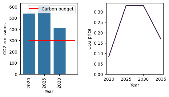
We can see a substantial reduction in CO2 emissions from 2020 to 2025, in line with the budget, driven by a sharp increase in the carbon price. Emissions are kept within the budget for the rest of the simulation.

Next, we will look at the MCACapacity.csv file, to see the investment decisions behind this outcome.

mca_capacity = pd.read_csv(
    "../tutorial-code/carbon-budget/1-carbon-budget/Results/MCACapacity.csv"
)

fig, axes = plt.subplots(1, 3)
all_years = mca_capacity["year"].unique()
for ax, (sector_name, sector_data) in zip(axes, mca_capacity.groupby("sector")):
    sector_capacity = sector_data.groupby(["year", "technology"]).sum().reset_index()
    sector_capacity.pivot(
        index="year", columns="technology", values="capacity"
    ).reindex(all_years).plot(kind="bar", stacked=True, ax=ax)
    ax.set_ylabel("Capacity (PJ)")
    ax.set_xlabel("Year")
    ax.set_title(f"{sector_name.capitalize()} Sector:", fontsize=10)
    ax.legend(title=None, prop={"size": 8})
    ax.tick_params(axis="both", labelsize=8)

fig.set_size_inches(8, 2.5)
fig.subplots_adjust(wspace=0.5)

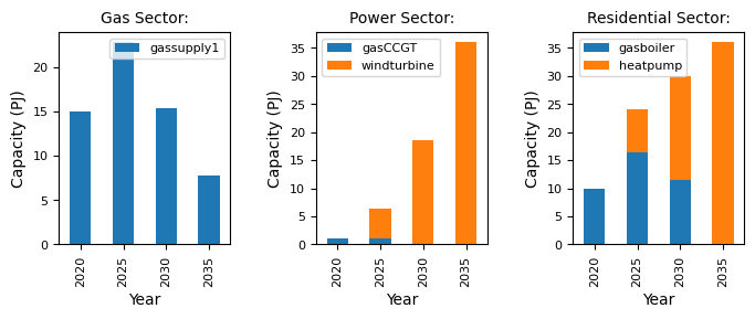
Compared to the default example, which has no carbon budget, we can see substantial investment in windturbine early on in the simulation. This can be explained by the increase in carbon price, which makes windturbine comparatively more attractive for investment than gasCCGT. As a result, we see a decline in the gas sector.

Have a play around with different carbon budget profiles to see the effect on emissions and investment decisions.